How to count unique values in Excel an easy way

The tutorial looks at how to leverage the new dynamic array functions to count unique values in Excel: formula to count unique entries in a column, with multiple criteria, ignoring blanks, and more.

A couple of years ago, we discussed various ways to count unique and distinct values in Excel. But like any other software program, Microsoft Excel continuously evolves, and new features appear with almost every release. Today, we will look at how counting unique values in Excel can be done with the recently introduced dynamic array functions. If you have not used any of these functions yet, you will be amazed to see how much simpler the formulas become in terms of building and convenience to use.

Note. All the formulas discussed in this tutorial rely on the UNIQUE function, which is only available in the latest version of Excel 365. If you are using Excel 2019, Excel 2016 or earlier, please check out this article for solutions.

• Count unique values in column
• Get count of unique values that occur only once
• Count unique rows
• Count unique entries ignoring blanks
• Count unique values with criteria
• Count unique values with multiple criteria

Count unique values in column

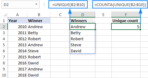
The easiest way to count unique values in a column is to use the UNIQUE function together with the COUNTA function: COUNTA(UNIQUE(range))

The formula works with this simple logic: UNIQUE returns an array of unique entries, and COUNTA counts all the elements of the array.

As an example, let's count unique names in the range B2:B10:

=COUNTA(UNIQUE(B2:B10))

The formula tells us that there are 5 different names in the winners list:

Tip. In this example, we count unique text values, but you can use this formula for other data types too including numbers, dates, times, etc.

Count unique values that occur just once

In the previous example, we counted all the different (distinct) entries in a column. This time, we want to know the number of unique records that occur only once. To have it done, build your formula in this way:

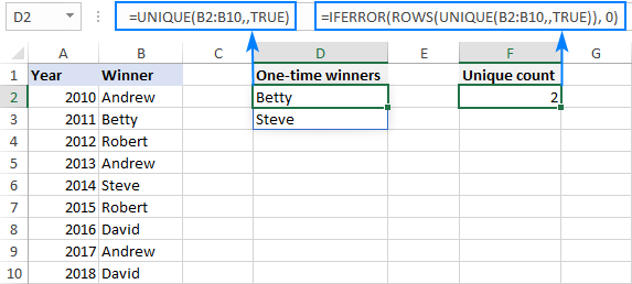
To get a list of one-time occurrences, set the 3rd argument of UNIQUE to TRUE:

UNIQUE(B2:B10,,TRUE))

To count the unique one-time occurrences, nest UNIQUE in the ROW function:

ROWS(UNIQUE(B2:B10,,TRUE))

Please note that COUNTA won't work in this case because it counts all non-blank cells, including error values. So, if no results are found, UNIQUE would return an error, and COUNTA would count it as 1, which is wrong!

To handle possible errors, wrap the IFERROR function around your formula and instruct it to output 0 if any error occurs:

=IFERROR(ROWS(UNIQUE(B2:B10,,TRUE)), 0)

As the result, you get a count based on the database concept of unique:

Count unique rows in Excel

Now that you know how to count unique cells in a column, any idea on how to find the number of unique rows?

Here's the solution:

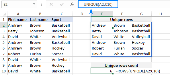
ROWS(UNIQUE(range))

The trick is to "feed" the entire range to UNIQUE so that it finds the unique combinations of values in multiple columns. After that, you simply enclose the formula in the ROWS function to calculate the number of rows.

For example, to count the unique rows in the range A2:C10, we use this formula:

=ROWS(UNIQUE(A2:C10))

Count unique entries ignoring blank cells

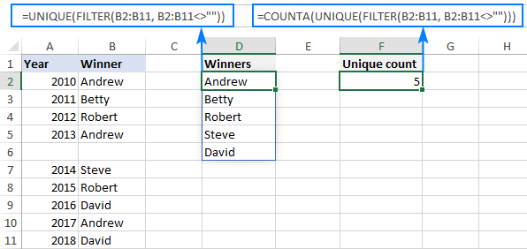
To count unique values in Excel ignoring blanks, employ the FILTER function to filter out empty cells, and then warp it in the already familiar COUNTA UNIQUE formula:

COUNTA(UNIQUE(FILTER(range, range<>"")))

With the source data in B2:B11, the formula takes this form:

=COUNTA(UNIQUE(FILTER(B2:B11, B2:B11<>"")))

The screenshot below shows the result:

Count unique values with criteria

To extract unique values based on certain criteria, you again use the UNIQUE and FILTER functions together as explained in this example. And then, you use the ROWS function to count unique entries and IFERROR to trap all kinds of errors and replace them with 0:

IFERROR(ROWS(UNIQUE(range, criteria_range=criteria))), 0)

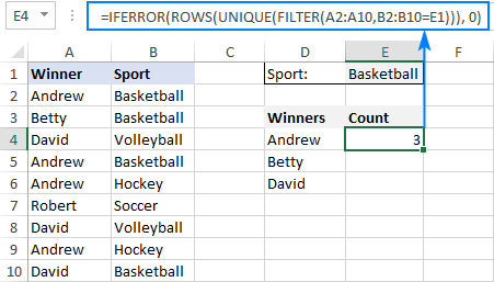
For example, to find how many different winners there are in a specific sport, use this formula:

=IFERROR(ROWS(UNIQUE(FILTER(A2:A10,B2:B10=E1))), 0)

Where A2:A10 is a range to search for unique names (range), B2:B10 are the sports in which the winners compete (criteria_range), and E1 is the sport of interest (criteria).

Count unique values with multiple criteria

The formula for counting unique values based on multiple criteria is pretty much similar to the above example, though the criteria are constructed a bit differently:

IFERROR(ROWS(UNIQUE(range, (criteria_range1=criteria1) * (criteria_range2=criteria2)))), 0)

Those who are curious to know the inner mechanics, can find the explanation of the formula's logic here: Find unique values based on multiple criteria.

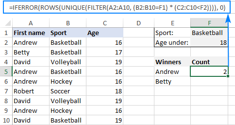
In this example, we are going to find out how many different winners there are in a specific sport in F1 (criteria 1) and under the age in F2 (criteria 2). For this, we are using this formula:

=IFERROR(ROWS(UNIQUE(FILTER(A2:A10, (B2:B10=F1) * (C2:C10<F2)))), 0)

Where A2:B10 is the list of names (range), C2:C10 are sports (criteria_range 1) and D2:D10 are ages (criteria_range 2).


That's how to count unique values in Excel with the new dynamic array functions. I am sure you appreciate how much simpler all the solutions become.