Calculating simple running totals in SQL Server
Introduction
One typical question is, how to calculate
running totals in SQL Server. There are several ways of doing it and this
article tries to explain a few of them.
Test
environment
First we need a table for the data. To keep things simple, let's
create a table with just an auto incremented id and a value field.
--------------------------------------------------------------------
--
table for test
--------------------------------------------------------------------
CREATE
TABLE RunTotalTestData (
id int not null identity(1,1) primary key,
value int not null
);
And populate it with some data:
--------------------------------------------------------------------
--
test data
--------------------------------------------------------------------
INSERT
INTO RunTotalTestData (value) VALUES (1);
INSERT
INTO RunTotalTestData (value) VALUES (2);
INSERT
INTO RunTotalTestData (value) VALUES (4);
INSERT
INTO RunTotalTestData (value) VALUES (7);
INSERT
INTO RunTotalTestData (value) VALUES (9);
INSERT
INTO RunTotalTestData (value) VALUES (12);
INSERT
INTO RunTotalTestData (value) VALUES (13);
INSERT
INTO RunTotalTestData (value) VALUES (16);
INSERT
INTO RunTotalTestData (value) VALUES (22);
INSERT
INTO RunTotalTestData (value) VALUES (42);
INSERT
INTO RunTotalTestData (value) VALUES (57);
INSERT
INTO RunTotalTestData (value) VALUES (58);
INSERT
INTO RunTotalTestData (value) VALUES (59);
INSERT
INTO RunTotalTestData (value) VALUES (60);
The scenario is to fetch a running
total when the data is ordered ascending by the id field.
Correlated
scalar query
One very traditional way is to use a
correlated scalar query to fetch the running total so far. The query could look
like:
--------------------------------------------------------------------
--
correlated scalar
--------------------------------------------------------------------
SELECT
a.id, a.value, (SELECT SUM(b.value)
FROM RunTotalTestData b
WHERE b.id <= a.id)
FROM RunTotalTestData
a
ORDER
BY a.id;
When this is run, the results are:
Copy Code
id value running total
-- ----- -------------
1 1 1
2 2 3
3 4 7
4 7 14
5 9 23
6 12 35
7 13 48
8 16 64
9 22 86
10 42 128
11 57 185
12 58 243
13 59 302
14 60 362
So there it was. Along with the actual row values, we have a
running total. The scalar query simply fetches the sum of the value field from the rows where the ID is equal or less than the
value of the current row. Let us look at the execution plan:
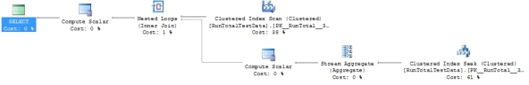
What happens is that the database
fetches all the rows from the table and using a nested loop, it again fetches
the rows from which the sum is calculated. This can also be seen in the
statistics:
Table
'RunTotalTestData'. Scan count 15, logical reads 30,
physical reads 0...
Using
join
Another variation is to use join.
Now the query could look like:
--------------------------------------------------------------------
--
using join
--------------------------------------------------------------------
SELECT
a.id, a.value, SUM(b.Value)
FROM RunTotalTestData
a,
RunTotalTestData b
WHERE
b.id <= a.id
GROUP
BY a.id, a.value
ORDER
BY a.id;
The results are the same but the technique is a bit different. Instead of
fetching the sum for each row, the sum is created by using a GROUP
BY clause. The rows are cross joined
restricting the join only to equal or smaller ID values in B. The plan:
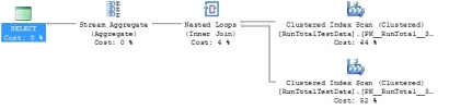
The plan looks somewhat different
and what actually happens is that the table is read
only twice. This can be seen more clearly with the statistics.
Table
'RunTotalTestData'. Scan count 2, logical reads 31...
The correlated scalar query has a
calculated cost of 0.0087873 while the cost for the join version is 0.0087618.
The difference isn't much but then again it has to be remembered that we're
playing with extremely small amounts of data.
Using
conditions
In real-life scenarios, restricting
conditions are often used, so how are conditions applied to these queries. The
basic rule is that the condition must be defined twice in both
of these variations. Once for the rows to fetch and the second time for
the rows from which the sum is calculated.
If we want to calculate the running
total for odd value numbers, the correlated scalar version could look like the
following:
--------------------------------------------------------------------
--
correlated scalar, subset
--------------------------------------------------------------------
SELECT
a.id, a.value, (SELECT SUM(b.value)
FROM RunTotalTestData b
WHERE b.id <= a.id
AND b.value % 2 = 1)
FROM RunTotalTestData a
WHERE
a.value % 2 = 1
ORDER
BY a.id;
The results are:
id value runningtotal
-- ----- ------------
1 1 1
4 7 8
5 9 17
7 13 30
11 57 87
13 59 146
And with the join version, it could
be like:
--------------------------------------------------------------------
--
with join, subset
--------------------------------------------------------------------
SELECT
a.id, a.value, SUM(b.Value)
FROM RunTotalTestData
a,
RunTotalTestData b
WHERE
b.id
<= a.id
AND a.value
% 2 = 1
AND b.value
% 2 = 1
GROUP
BY a.id, a.value
ORDER
BY a.id;
When actually
having more conditions, it can be quite painful to maintain the conditions
correctly. Especially if they are built dynamically.
Calculating
running totals for partitions of data
If the running total needs to be
calculated to different partitions of data, one way to do it is just to use
more conditions in the joins. For example, if the running totals would be
calculated for both odd and even numbers, the correlated scalar query could
look like:
--------------------------------------------------------------------
--
correlated scalar, partitioning
--------------------------------------------------------------------
SELECT
a.value%2, a.id, a.value, (SELECT SUM(b.value)
FROM RunTotalTestData b
WHERE b.id <= a.id
AND b.value%2 = a.value%2)
FROM RunTotalTestData
a
ORDER
BY a.value%2, a.id;
The results:
even id value running total
---- -- ----- -------------
0 2 2 2
0 3 4 6
0 6 12 18
0 8 16 34
0 9 22 56
0 10 42 98
0 12 58 156
0 14 60 216
1 1 1 1
1 4 7 8
1 5 9 17
1 7 13 30
1 11 57 87
1 13 59 146
So now the partitioning condition is
added to the WHERE
clause of the scalar query. When using the join version, it could be similar to:
--------------------------------------------------------------------
--
with join, partitioning
--------------------------------------------------------------------
SELECT
a.value%2, a.id, a.value, SUM(b.Value)
FROM RunTotalTestData
a,
RunTotalTestData b
WHERE
b.id <=
a.id
AND b.value%2 = a.value%2
GROUP
BY a.value%2, a.id, a.value
ORDER
BY a.value%2, a.id;
With
SQL Server 2012
SQL Server 2012 makes life much more simpler. With this version, it's possible to define an ORDER
BY clause in the OVER clause.
So to get the running total for all rows, the query would
look:
--------------------------------------------------------------------
--
Using OVER clause
--------------------------------------------------------------------
SELECT
a.id, a.value, SUM(a.value)
OVER (ORDER BY a.id)
FROM RunTotalTestData
a
ORDER
BY a.id;
The syntax allows to define the
ordering of the partition (which in this example includes all rows) and the
summary is calculated in that order.
To define a condition for the data,
it doesn't have to be repeated anymore. The running total for odd numbers would
look like:
--------------------------------------------------------------------
--
Using OVER clause, subset
--------------------------------------------------------------------
SELECT
a.id, a.value, SUM(a.value)
OVER (ORDER BY a.id)
FROM RunTotalTestData
a
WHERE
a.value % 2 = 1
ORDER
BY a.id;
And finally, partitioning would be:
--------------------------------------------------------------------
--
Using OVER clause, partition
--------------------------------------------------------------------
SELECT
a.value%2, a.id, a.value, SUM(a.value)
OVER (PARTITION BY a.value%2 ORDER BY a.id)
FROM RunTotalTestData
a
ORDER
BY a.value%2, a.id;
What about the plan? It's looking
very different. For example, the simple running total for all rows looks like:
![]()
And the statistics:
Table
'Worktable'. Scan count 15, logical reads 85, physical reads 0...
Table
'RunTotalTestData'. Scan count 1, logical reads 2,
physical reads 0...
Even though the scan count looks
quite high at first glance, it isn't targeting the actual table but a
worktable. The worktable is used to store intermediate results which are then
read in order to create the calculated results.
The calculated cost for this query
is now 0.0033428 while previously with the join version, it was 0.0087618.
Quite an improvement.
References